Understanding technology choices through computing tasks

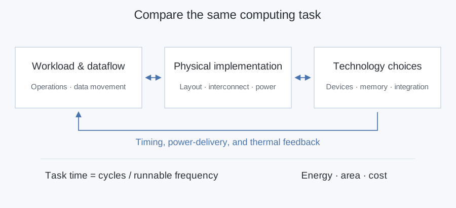
Suppose we want to improve a matrix-multiplication engine. We could add compute units, bring memory closer, use faster devices, or change how the dies are stacked. Each choice also changes communication, power delivery, and heat. To understand which choice helps, we need to follow the same workload through its physical implementation.

This question framed our ICCC 2026 talk on system–technology co-optimization (STCO). We use physical design to connect what an architecture is meant to do with how devices and manufacturing technologies allow us to build it. Here, we look at two examples from our work: power-delivery optimization and multi-reticle chiplet placement.

Start with the same computing task

We begin by fixing the matrix dimensions, numerical precision, and batch size. In a systolic array, operands are reused as they move between neighboring multiply–accumulate units. Increasing parallelism can reduce compute cycles, but the memory system must supply data quickly enough. Moving memory onto another tier changes the communication distance, vertical connections, and distribution of heat.

The task time depends on both the required cycles and the usable frequency:

T_task = N_cycles / f_run.

Here, the cycle count includes computation and waiting for data. The running frequency depends on implemented signal paths, supply voltage, and temperature. A dataflow that saves cycles can lose that benefit if its physical implementation forces a lower clock rate.

To compare these choices, we need results from logic mapping, placement and routing, and analysis of interconnect, power delivery, and heat. We can then use those results to revisit our choices of parallelism, memory placement, and technology.

Task mapping and technology choices meet in a physical implementation, whose timing, power, and thermal behavior determines task time and energy. — We compare system and technology choices by following the same task through implementation and looking at its time, energy, area, and cost.

Power delivery changes the usable frequency

In a dense chiplet system, many cores switching together create sharp current peaks. Parasitics in microbumps, interposer metal, and through-silicon vias (TSVs) affect the power network’s response. Voltage droop weakens transistor drive and increases gate delay, limiting the frequency at which the architecture can run.

In CNE-PDN, we connect these effects to layout decisions through a component-level model. We use electromagnetic simulation to fit equivalent resistance, inductance, and capacitance. For fixed TSV structures, we reuse the fitted parameters; for changing metal geometries, we predict them with a neural network. We then assemble the components according to the candidate layout.

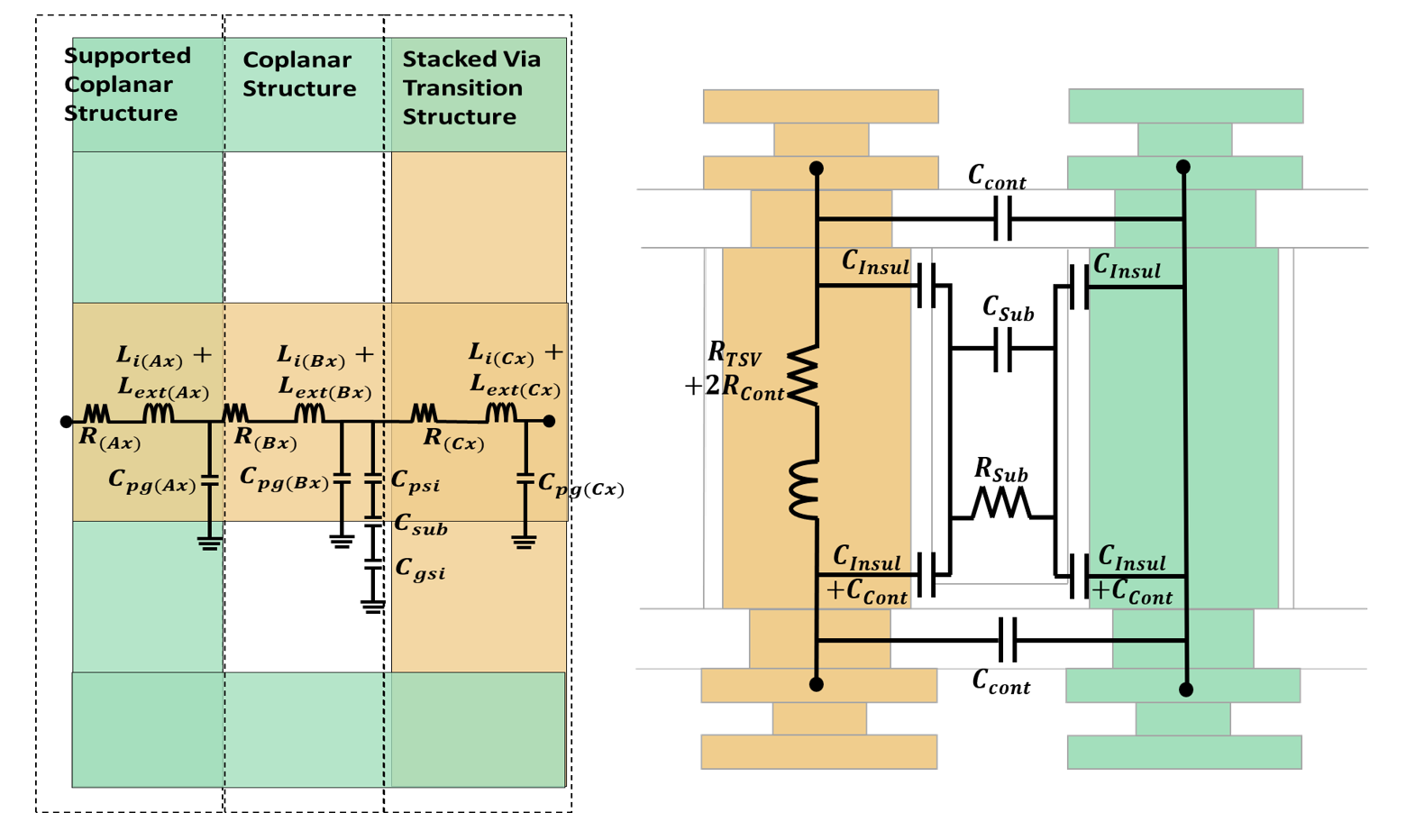
Equivalent resistance, inductance, and capacitance models for horizontal interposer metal and vertical TSV structures. — CNE-PDN represents metal segments and TSVs with coupled circuit components, preserving their geometry and connections during layout evaluation.

From the assembled network’s impedance and the switching-current waveform, we obtain the voltage response. We average the voltage over the switching window and use it to estimate the supply-limited frequency. This lets us evaluate how a change in metal dimensions or TSV locations affects the frequency at which the system can run.

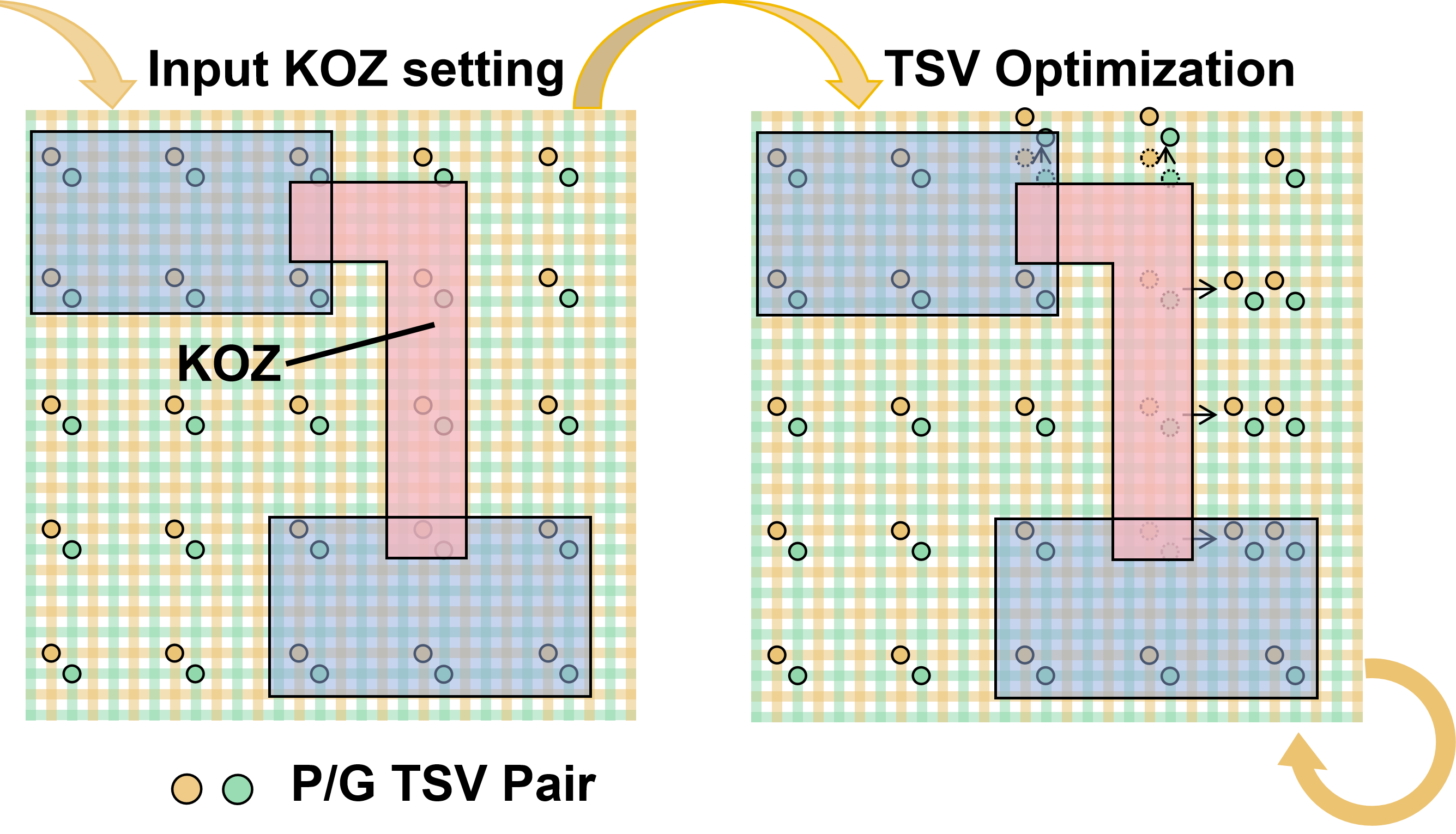
After fitting and training, we can evaluate a candidate in about eight seconds, compared with roughly fifty minutes for the HFSS–SPICE flow. We can search over metal dimensions and TSV placement together, accounting for routing congestion and keep-out regions. In the CPU/GPU/HBM design we evaluated, changing TSV locations raised the estimated supply-limited frequency from 1.935 to 2.029 GHz while keeping the chiplet composition and metal dimensions fixed.

TSV positions adjusted on a power grid around chiplet footprints and a keep-out region. — In CNE-PDN, we adjust supply and ground TSV positions along the grid. Blue regions are chiplets; pink marks a TSV keep-out zone.

Manufacturing changes the feasible layout

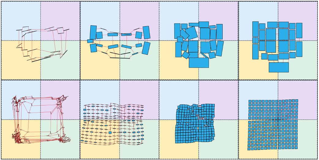
In ULTRA-2.5D, we study how manufacturing constraints shape chiplet placement. Larger chiplet systems may need interposers spanning several lithographic exposure fields. Stitching these fields introduces alignment effects and different routing rules at their boundaries.

These rules affect where chiplets can go and how their pins connect. A chiplet may bridge adjacent fields so that critical connections remain within one field. Its rotation or flip can determine whether that arrangement is possible. Manufacturing constraints therefore change the placement search itself.

We account for these constraints by combining multi-reticle partitioning, differentiable position-and-orientation optimization, and legalization. ULTRA-2.5D completed all seven benchmarks, including a case with 1,225 chiplets. Across the five cases also completed by ATPlace2.5D, the baseline’s total half-perimeter wirelength was 1.40 times ours, using the geometric mean. By including the reticle structure in the optimization, we can place chiplets with both their connections and the manufacturing rules in view.

ULTRA-2.5D placement snapshots for 22 and 225 chiplets, from initial positions to final layouts across four reticle regions. — ULTRA-2.5D placement snapshots for 22 and 225 chiplets. Background colors distinguish reticle regions; successive panels show the placement process.

Bringing the choices together

We can use the same reasoning to think about device and integration choices. Device models determine cell delay, power, and area; metal and bonding rules determine interconnect loads. Mapping and physical design turn those properties into signal paths, while power and thermal analysis tell us which operating conditions are usable.

Memory bandwidth, bonding density, and cooling also affect which architecture is worthwhile. More compute units need more data and power. Closer memory can shorten communication while changing thermal paths. We therefore come back to the computing task: how long does it take, how much energy does it use, and what area and manufacturing cost does the design require?

With CNE-PDN, we use a physical model to guide layout decisions toward a higher usable frequency. With ULTRA-2.5D, we bring manufacturing rules into large-scale chiplet placement. Both give us a way to see how system and technology choices play out in a physical design—and to use that feedback when deciding what to change next.

Based on Keren Zhu's ICCC 2026 talk, System–Technology Co-design for Three-Dimensional Chips. Related work: CNE-PDN (ICCAD 2026; code) and ULTRA-2.5D (IEEE TCAD 2026).